Atoms and the Periodic Table IV: The Wave Function of Hydrogen Atom
In this section, we are going to apply the basic rule of quantum mechanics, the Schrodinger's equation, for hydrogen atom. From quantum mechanics, we can predict the behaviour of electron in hydrogen atom, which is the where the electron likely to be. The hydrogen atom is chosen for this discussion due to hydrogen atom is the simplest system (1 electron and 1 proton), and the solution for hydrogen atom lies on the Schrodinger's equation.

Firstly, we need to consider the interaction of electron and proton. The attraction between proton and electron is basically the coloumbic force of the charges particle. Besides that, we also assume that H atom is spherically symmetric system which means all the forces are the same in every point at the sphere. The position at the sphere can be described as as cartesian coordinate (x, y, z coordinate). However, it might be more convenient to develop another system for spherical system, which is spherical polar coordinate (r, θ, ϕ).
 For polar coordinate, r stands for the distance between a certain point from the origin (radial coordinate) and the value for r is 0 < r < ∞. θ is the co-latitude angle which is measured the angle between the north pole and the r vector, so the value of θ is from 0 < θ < π. The last parameter is ϕ, which is the longitude angle.
ϕ is measured from the x-axis, so the value of ϕ is from 0 < ϕ < 2π. In the other sides, the cartesian coordinates the value of x, y, and z are from -∞ < r < ∞.
For the H atom, since it has 3 dimensional system, so it has three degrees of freedom which in polar coordinate as r, θ, ϕ. Then, the polar coordinate is translated into 3 quantum numbers, n (principal quantum number), l (orbital angular momentum quantum number), and ml (magnetic quantum number).
The principal quantum number (n) determines the energy of each orbit as we have discussed before and the value of n = 1,2,3, ..., n. Then, orbital angular momentum quantum number (l) determines the shape of orbital and the value of l is depend on n which l = 0, 1, 2, ..., (n-1). Lastly, the magnetic quantum number determines the orientation of the electron in orbital and the value ml of run from l,0, to -l. Moreover, the total number of ml that possible can be summarised as 2l + 1. Since, the wave function is a function of position and in H atom is based on 3 quantum numbers, so we can rewrite our Schrodinger's equation as:
 Fortunately, based on the equation above energy only depends on the n in H atom, which have a degenerates state. Therefore, for the same n would have the same energy. Moreover, if we have fixed n the number of the degenerates states is:
 Now, if we apply the equation above we can get:
From the table above, the shell represents the fixed n and all has the same energy for H atom for the same n. Then, the subshell represent the value of l and it represent the shape of the wave function. For l = 0 is known as the s (sharp)-type, l = 1 is the p (principal)-type, l = 2 is the d (diffuse)-type, and l = 3 is the f (fundamental)-type; the name of the l is just come from the spectra. The orbital itself basically represents the orientation (point) of the electron and also represents the wave function for 1 electron. Therefore, from the table above 1s is the wave function at the lowest energy level and each orbital represent a wave function.
The Schrodinger's equation for H atom basically is a triumph for describing the atom. It proves the discrete energy and also predict the value of Rydberg's constant. Moreover, the Schrodinger's equation also strengthen the Bohr's model with the explanation which electron behave as a wave, which lead to the electron distribution (ψ2).
If we move to our original problem to define the probability of electron, so we need to apply the Schrodinger's equation. Basically, ψ is a position of wave function which is the orbital and ψ2 is the electron distribution which is the probability density. Therefore, if we multiply the with a change of volume (dV), we can get the probability. Furthermore, if we integrate to all the point at space the function of ψ2dV we can get the probability is 1. The value of probability is from 0 (never happen) to 1 (certainly happen).
 From the equation above, it means you will found electron in the space.
Now, we can move to the problem how to plot our function. As we have discussed previously, the wave function consists 3 different parameters, the cartesian coordinate and the spherical polar coordinate are used interchangeably. However, there is a problem with the function to be drawn in as graph and it comes from the 3 parameters of the function (x, y, z).
To make the problem more clearly, let take the example if we have f(x) as our function. The value of f(x) depends on the x and we can plot as the x-axis and f(x) as the y-axis. Then, if we have a function f(x, y) which values of f(x, y) depends on the value x and y, so we can plot the function as x-axis, y-axis, and f(x, y) as the z-axis. Now, the problem is if we have a function of f(x, y, z) similar with our wave function, we can plot the x-axis, y-axis, and z-axis, but where we should put the f(x, y, z). Therefore, the solution is we can split our function, so we can put the function on the graph. Before, we split our wave function, it is better to know the term that will be used to plot our wave function.
As, the electron behaves as a wave, so in some points on the wave it will cross the x-axis which means the ψ=0, so at that point we will not be able to find the electron. The point which it is impossible to find the electron (p = 0) is called by nodal point.
For the same measurement of length, if a wave has more nodal points it means the wave has shorter λ. Therefore, if a wave has shorter λ, it means it has higher momentum and also higher energy.
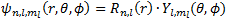
Now, to split our wave function, we should define our wave function first. The variable of the wave function can be separated into 2 function. Firstly, we can define the wave function as radial function [R(r)] which the values depends on the n and l. Secondly, we can define our wave function as the angular function [Y(θ, ϕ)] and the values depends on l and ml. Therefore, the wave function can be written as:
 Therefore, we can draw our wave function and we can start from the wave function as radial function.
Firstly, we need to consider the interaction of electron and proton. The attraction between proton and electron is basically the coloumbic force of the charges particle. Besides that, we also assume that H atom is spherically symmetric system which means all the forces are the same in every point at the sphere. The position at the sphere can be described as as cartesian coordinate (x, y, z coordinate). However, it might be more convenient to develop another system for spherical system, which is spherical polar coordinate (r, θ, ϕ).

ϕ is measured from the x-axis, so the value of ϕ is from 0 < ϕ < 2π. In the other sides, the cartesian coordinates the value of x, y, and z are from -∞ < r < ∞.
For the H atom, since it has 3 dimensional system, so it has three degrees of freedom which in polar coordinate as r, θ, ϕ. Then, the polar coordinate is translated into 3 quantum numbers, n (principal quantum number), l (orbital angular momentum quantum number), and ml (magnetic quantum number).
The principal quantum number (n) determines the energy of each orbit as we have discussed before and the value of n = 1,2,3, ..., n. Then, orbital angular momentum quantum number (l) determines the shape of orbital and the value of l is depend on n which l = 0, 1, 2, ..., (n-1). Lastly, the magnetic quantum number determines the orientation of the electron in orbital and the value ml of run from l,0, to -l. Moreover, the total number of ml that possible can be summarised as 2l + 1. Since, the wave function is a function of position and in H atom is based on 3 quantum numbers, so we can rewrite our Schrodinger's equation as:
Shells
|
Subshells
|
Orbital
|
||
K
|
n = 1
|
l = 0
|
ml = 0
(1 value) |
1s
|
L
|
n = 2
|
l = 0
|
ml = 0
(1 value) |
2s
|
l =1
|
ml = -1, 0, 1
(3 values) |
2p
|
||
From the table above, the shell represents the fixed n and all has the same energy for H atom for the same n. Then, the subshell represent the value of l and it represent the shape of the wave function. For l = 0 is known as the s (sharp)-type, l = 1 is the p (principal)-type, l = 2 is the d (diffuse)-type, and l = 3 is the f (fundamental)-type; the name of the l is just come from the spectra. The orbital itself basically represents the orientation (point) of the electron and also represents the wave function for 1 electron. Therefore, from the table above 1s is the wave function at the lowest energy level and each orbital represent a wave function.
The Schrodinger's equation for H atom basically is a triumph for describing the atom. It proves the discrete energy and also predict the value of Rydberg's constant. Moreover, the Schrodinger's equation also strengthen the Bohr's model with the explanation which electron behave as a wave, which lead to the electron distribution (ψ2).
If we move to our original problem to define the probability of electron, so we need to apply the Schrodinger's equation. Basically, ψ is a position of wave function which is the orbital and ψ2 is the electron distribution which is the probability density. Therefore, if we multiply the with a change of volume (dV), we can get the probability. Furthermore, if we integrate to all the point at space the function of ψ2dV we can get the probability is 1. The value of probability is from 0 (never happen) to 1 (certainly happen).
Now, we can move to the problem how to plot our function. As we have discussed previously, the wave function consists 3 different parameters, the cartesian coordinate and the spherical polar coordinate are used interchangeably. However, there is a problem with the function to be drawn in as graph and it comes from the 3 parameters of the function (x, y, z).
To make the problem more clearly, let take the example if we have f(x) as our function. The value of f(x) depends on the x and we can plot as the x-axis and f(x) as the y-axis. Then, if we have a function f(x, y) which values of f(x, y) depends on the value x and y, so we can plot the function as x-axis, y-axis, and f(x, y) as the z-axis. Now, the problem is if we have a function of f(x, y, z) similar with our wave function, we can plot the x-axis, y-axis, and z-axis, but where we should put the f(x, y, z). Therefore, the solution is we can split our function, so we can put the function on the graph. Before, we split our wave function, it is better to know the term that will be used to plot our wave function.
As, the electron behaves as a wave, so in some points on the wave it will cross the x-axis which means the ψ=0, so at that point we will not be able to find the electron. The point which it is impossible to find the electron (p = 0) is called by nodal point.
 |
| nodal point => where f(x) =0 |
Now, to split our wave function, we should define our wave function first. The variable of the wave function can be separated into 2 function. Firstly, we can define the wave function as radial function [R(r)] which the values depends on the n and l. Secondly, we can define our wave function as the angular function [Y(θ, ϕ)] and the values depends on l and ml. Therefore, the wave function can be written as:
Comments